What Is the Welfare State?

A thorough guide to the welfare state — its Bismarckian origins, Esping-Andersen's three worlds typology, the Beveridge Report, Nordic universalism, the US welfare state's fragmented character, the economics of social insurance, evidence on poverty reduction, and the political economy of retrenchment.

What Is the Simulation Hypothesis?

Nick Bostrom's simulation argument explained: the trilemma, the physics objections, the consciousness problem, and what it would mean if our reality were computed.

How Does Machine Learning Work?

By Kalenux Team

Published 2026-04-14 · Updated 2026-04-15

✓ Fact-checked by the Kalenux editorial team

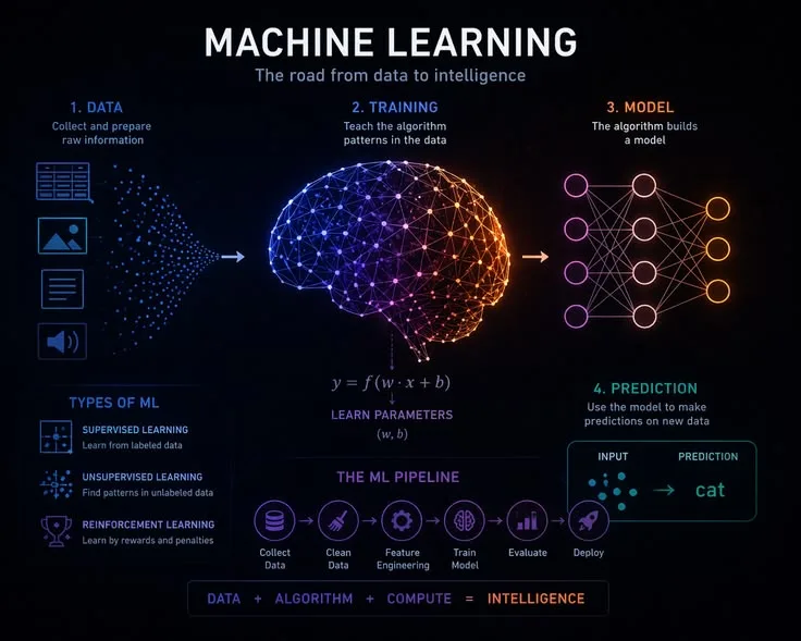
Machine learning is a branch of artificial intelligence in which computer systems learn to perform tasks by finding patterns in data rather than following explicitly programmed rules. Instead of writing code that says "if an email contains the word free and the phrase click here, mark it as spam," a machine learning system is shown thousands of examples of spam and legitimate email, and it figures out the distinguishing patterns on its own. The result is a mathematical model -- a set of learned parameters -- that can classify new emails with high accuracy based on what it learned from examples.

This approach has proven transformative because many real-world problems are too complex for hand-coded rules. Recognizing faces in photographs, translating between languages, diagnosing tumors from medical images, recommending content, predicting weather patterns, and generating human-like text all involve patterns that are extraordinarily difficult to articulate as explicit rules but can be learned from large datasets. Machine learning does not understand these tasks the way a human does -- it learns statistical associations that are predictively useful.

The field has grown from a niche area of computer science to one of the most consequential technologies of the 21st century. According to a 2024 report by McKinsey Global Institute, AI and machine learning are projected to contribute between $17.1 trillion and $25.6 trillion to the global economy by 2030. Stanford's 2024 AI Index Report documented that the number of AI-related publications doubled between 2018 and 2023, and industry investment in AI reached $91.9 billion in 2022 alone.

"A computer program is said to learn from experience E with respect to some class of tasks T and performance measure P, if its performance at tasks in T, as measured by P, improves with experience E." -- Tom Mitchell, Machine Learning (1997)

This article explains the foundational mechanics: what training data is, how features shape what a model can learn, the three major paradigms (supervised, unsupervised, and reinforcement learning), how neural networks function, what overfitting is and why it matters, and how models continue to improve with feedback and additional data.

Key Definitions

Before diving into how machine learning works, it helps to establish the core vocabulary. These terms appear throughout the field and in this article:

Training data: The dataset used to fit a machine learning model. It contains the examples the algorithm learns from. In supervised learning, training data includes labels -- the correct answers the model is trying to predict.

Feature: An individual measurable input variable used by a model. In a house price prediction model, features might include square footage, number of bedrooms, neighborhood, and year of construction. The choice and quality of features profoundly affects what a model can learn.

Model: The mathematical structure -- defined by its architecture and learned parameters -- that takes input data and produces an output (a prediction, classification, or decision). A model's parameters are adjusted during training to improve accuracy.

Loss function: A mathematical measure of how far the model's predictions are from the correct answers. Training consists of minimizing this function -- finding the parameter values that make predictions as close to reality as possible.

Generalization: A model's ability to perform well on new data it has not seen during training. Good generalization is the ultimate goal of machine learning. A model that memorizes training data but fails on new examples has learned nothing useful.

Hyperparameters: Settings chosen by the human practitioner before training begins -- learning rate, number of layers, regularization strength. Unlike model parameters (which are learned from data), hyperparameters are set by the engineer and tuned through experimentation.

Training Data: The Foundation of All Machine Learning

What Training Data Is and Why It Matters

No machine learning system learns from nothing. Every model requires data, and the quality and quantity of that data largely determines the quality of the model. As Pedro Domingos wrote in The Master Algorithm (2015): "It's not who has the best algorithm that wins. It's who has the most data."

Training data consists of examples -- typically input-output pairs in supervised learning -- that the algorithm uses to adjust its parameters. For an image classification system, training data might consist of millions of photographs labeled with the objects they contain. For a language model like GPT-4, it is hundreds of billions of words of text from books, websites, and other sources. For a fraud detection system, it is historical transaction records with labels indicating which transactions were fraudulent.

The scale of modern training datasets is extraordinary. ImageNet, the dataset that catalyzed the deep learning revolution, contains over 14 million labeled images across more than 20,000 categories. It was assembled through years of work led by Fei-Fei Li at Stanford, who recruited over 25,000 workers through Amazon's Mechanical Turk to label the images. GPT-3 was trained on approximately 570 gigabytes of text data -- roughly equivalent to the contents of 400,000 books.

Data Quality Matters More Than Quantity

Machine learning researchers often cite the principle of "garbage in, garbage out." A model trained on biased, incorrect, or unrepresentative data will learn biased, incorrect patterns -- and it will apply those patterns with confidence because it has no way to know its training data was flawed.

This is not a theoretical concern. Joy Buolamwini, a researcher at MIT Media Lab, demonstrated in her landmark 2018 paper "Gender Shades" (co-authored with Timnit Gebru) that commercial facial recognition systems from IBM, Microsoft, and Face++ had error rates for dark-skinned women that were up to 34.7 percent higher than for light-skinned men. The cause was not algorithmic malice -- it was training data that disproportionately represented lighter-skinned faces.

Similarly, ProPublica's 2016 investigation of the COMPAS criminal recidivism prediction algorithm found that it was significantly more likely to falsely label Black defendants as high-risk than white defendants. The algorithm had learned patterns from historical criminal justice data that reflected existing racial disparities in policing and sentencing.

Curating diverse, representative, accurately labeled training data is often the hardest and most time-consuming part of building a machine learning system. Andrew Ng, co-founder of Google Brain and a leading figure in AI education, has argued that the field needs to shift from "model-centric" to "data-centric" AI -- focusing more effort on improving data quality rather than developing ever-more-complex algorithms.

Features and Feature Engineering

Raw data is rarely in a form that a model can directly use. Feature engineering is the process of selecting, transforming, and creating input variables that best represent the underlying information for the prediction task.

For a loan default prediction model, raw data might include transaction histories, income records, and credit history. Feature engineering might produce derived variables: debt-to-income ratio, number of late payments in the past 12 months, total credit utilization percentage, and variance in monthly spending. These engineered features capture domain knowledge and can dramatically improve model performance -- sometimes more than switching to a more sophisticated algorithm.

Deep learning has reduced the need for manual feature engineering in some domains. Convolutional neural networks (CNNs), for example, learn relevant features from raw image pixels automatically -- early layers detect edges, middle layers detect textures and shapes, and later layers recognize complex objects. This ability to learn features directly from raw data, rather than requiring human engineers to design them, is one of the key advantages of deep learning. However, feature engineering remains critical in many business and scientific applications where domain knowledge is essential and data is limited.

The Three Major Learning Paradigms

Supervised Learning: Learning from Labeled Examples

Supervised learning is the most widely used form of machine learning in commercial applications. It requires labeled training data: every example has an input (features) and a known correct output (label). The algorithm learns to map inputs to outputs by minimizing prediction errors across the training set.

Two broad categories of supervised tasks exist:

Classification: The output is a discrete category. Spam detection (spam or not spam), medical diagnosis (malignant or benign), sentiment analysis (positive, negative, or neutral), and image recognition (cat, dog, car, tree) are classification tasks. A classifier outputs either a predicted class label or a probability distribution across possible classes.

Regression: The output is a continuous numerical value. Predicting house prices, forecasting sales revenue, estimating patient risk scores, and predicting stock returns are regression tasks. The model outputs a number rather than a category.

Key algorithms used in supervised learning include:

Linear and logistic regression -- among the oldest and most interpretable methods, still widely used as baselines
Decision trees and random forests -- Leo Breiman developed random forests in 2001, combining many decision trees to reduce variance and improve prediction accuracy. Random forests remain among the most popular algorithms in applied machine learning.
Gradient boosting (XGBoost, LightGBM, CatBoost) -- developed from Jerome Friedman's foundational work, gradient boosting builds trees sequentially, with each tree correcting the errors of its predecessors. XGBoost, created by Tianqi Chen in 2016, has won more Kaggle machine learning competitions than any other algorithm.
Support vector machines -- effective for classification tasks, particularly with smaller datasets
Neural networks -- the foundation of deep learning, discussed in detail below

Unsupervised Learning: Finding Structure Without Labels

Unsupervised learning works with unlabeled data, seeking to discover structure or patterns without predefined correct answers. This is useful when labeled data is scarce or expensive to obtain, or when the goal is exploration rather than prediction.

Clustering groups similar data points together. The k-means algorithm, among the simplest and most widely used, assigns data points to k clusters by minimizing the distance from each point to its cluster center. Clustering is used in customer segmentation (identifying natural groupings of customers by behavior), document grouping, anomaly detection (finding transactions that do not fit any normal cluster, potentially indicating fraud), and genomic analysis.

Dimensionality reduction finds lower-dimensional representations of high-dimensional data while preserving as much information as possible. Principal Component Analysis (PCA) finds the directions of maximum variance. t-SNE (developed by Laurens van der Maaten and Geoffrey Hinton, 2008) and UMAP (McInnes, Healy, and Melville, 2018) are used to visualize high-dimensional data in two or three dimensions. These methods are essential in genomics, where datasets might have tens of thousands of features per sample, and in natural language processing, where word embeddings exist in hundreds of dimensions.

Generative models learn the underlying distribution of training data well enough to generate new examples. Generative Adversarial Networks (GANs), developed by Ian Goodfellow in a 2014 paper that is now one of the most cited in machine learning history, use two competing networks -- a generator that creates fake examples and a discriminator that tries to distinguish them from real ones -- to produce increasingly realistic outputs. GANs can generate photorealistic faces, create art, and synthesize medical images for research when real patient data is scarce.

Reinforcement Learning: Learning from Rewards and Penalties

Reinforcement learning (RL) involves an agent that learns to make decisions by interacting with an environment. The agent takes actions, receives rewards or penalties based on the outcomes, and adjusts its policy (its strategy for choosing actions) to maximize cumulative reward over time.

There is no labeled training data in the traditional sense. The learning signal comes entirely from the reward function -- a mathematical specification of what success looks like. The agent must explore many actions and observe their consequences before converging on good policies, making RL computationally expensive but extraordinarily powerful in the right domains.

The landmark achievements of reinforcement learning include:

DeepMind's AlphaGo (Silver et al., 2016) defeated world champion Lee Sedol at Go -- a game with more possible board positions than atoms in the observable universe -- using a combination of deep neural networks and reinforcement learning
AlphaZero (Silver et al., 2017) mastered Chess, Go, and Shogi from scratch, learning solely through self-play with no human knowledge beyond the rules
OpenAI Five (2019) defeated professional teams at Dota 2, a complex multiplayer video game requiring long-term strategy and real-time decision-making
RLHF (Reinforcement Learning from Human Feedback) is the technique used to fine-tune large language models like ChatGPT, aligning their outputs with human preferences

Paradigm Comparison

Paradigm	Training Data	Goal	Example Applications	Key Algorithms
Supervised	Labeled (input + correct output)	Learn input-output mapping	Spam detection, medical diagnosis, price prediction	Neural networks, gradient boosting, SVM
Unsupervised	Unlabeled	Discover hidden structure	Customer segmentation, anomaly detection, topic modeling	k-means, PCA, autoencoders
Reinforcement	Environment rewards/penalties	Maximize cumulative reward	Game-playing AI, robotics, recommendation systems	Q-learning, policy gradients, PPO
Self-supervised	Unlabeled (labels derived from data itself)	Learn general representations	Language models, image pretraining	BERT, GPT, SimCLR
Semi-supervised	Small labeled + large unlabeled	Leverage both data types	Low-resource NLP, medical imaging	Label propagation, pseudo-labeling

Modern AI systems often combine paradigms: large language models are self-supervised pretrained, then fine-tuned with supervised learning and reinforcement learning from human feedback (RLHF).

How Neural Networks Work: The Engine of Deep Learning

Structure: Layers, Neurons, and Weights

A neural network is organized into layers. The input layer receives raw features. One or more hidden layers transform the input through learned operations. The output layer produces the prediction.

Each neuron in a layer receives inputs from all neurons in the previous layer. It multiplies each input by a learned weight, sums the weighted inputs, adds a bias term, and applies a nonlinear activation function (such as ReLU -- Rectified Linear Unit, which outputs zero for negative inputs and the input itself for positive inputs). The result is passed to the next layer.

Mathematically, a single neuron computes:

output = f(w1 * x1 + w2 * x2 + ... + wn * xn + b)

where w are weights, x are inputs, b is a bias, and f is the activation function. The power of neural networks comes from stacking many such layers: each layer learns increasingly abstract representations of the input data. An image recognition network's early layers might detect edges, middle layers detect textures and shapes, and later layers recognize objects like faces, cars, or buildings.

The term "neural network" is borrowed from neuroscience -- the artificial neurons are loosely inspired by biological neurons that receive signals, process them, and fire outputs. However, the resemblance is largely metaphorical. Modern neural networks are mathematical optimization machines, not biological simulations. As Yann LeCun, chief AI scientist at Meta, has noted: "calling them neural networks is a bit of a misnomer."

Training: Forward Pass and Backpropagation

Training a neural network involves two steps repeated millions of times:

Forward pass: Input data flows through the network layer by layer, with each layer applying its weights and activation functions, producing a prediction at the output layer.

Backward pass (backpropagation): The prediction error is calculated using the loss function (for example, how far the predicted house price is from the actual price). Using calculus -- specifically the chain rule -- the error is attributed backward through all layers, determining how much each weight contributed to the error. Each weight is then adjusted slightly in the direction that reduces the error. The size of each adjustment is controlled by the learning rate -- too large and the network overshoots; too small and learning takes impractically long.

Backpropagation was not invented once but developed independently by several researchers. The version most used today was popularized by David Rumelhart, Geoffrey Hinton, and Ronald Williams in their seminal 1986 paper "Learning Representations by Back-Propagating Errors" in Nature. It remains the foundational training algorithm for essentially all neural networks.

The optimization algorithm that performs weight updates is most commonly stochastic gradient descent (SGD) or variants like Adam, developed by Diederik Kingma and Jimmy Ba in 2014. Adam adapts the learning rate for each parameter individually, often converging faster than vanilla SGD. Training on large datasets requires processing examples in mini-batches -- updating weights after each batch of, say, 32 or 256 examples rather than after the entire dataset.

Deep Learning: Many Layers, Hierarchical Representations

Deep learning refers to neural networks with many hidden layers -- sometimes dozens or hundreds. Deep networks can learn hierarchical representations: early layers detect simple features, intermediate layers combine these into increasingly complex patterns, and later layers recognize high-level concepts.

The deep learning revolution accelerated dramatically in 2012 when a team led by Geoffrey Hinton submitted AlexNet to the ImageNet Large Scale Visual Recognition Challenge (ILSVRC). AlexNet achieved a top-5 error rate of 15.3 percent -- compared to 26.2 percent for the second-place entry, a gap so large it stunned the computer vision community. This breakthrough, enabled by GPU computing and the large labeled ImageNet dataset, launched the modern era of deep learning.

Key deep learning architectures include:

Convolutional Neural Networks (CNNs): Specialized for grid-like data (images, video). Developed by Yann LeCun in the 1990s, they use shared weights that slide across the input, dramatically reducing parameters while capturing spatial patterns.
Recurrent Neural Networks (RNNs) and LSTMs: Designed for sequential data (text, time series). Long Short-Term Memory networks, developed by Sepp Hochreiter and Jurgen Schmidhuber in 1997, solved the vanishing gradient problem that prevented earlier RNNs from learning long-range dependencies.
Transformers: Introduced by Vaswani et al. in the 2017 paper "Attention Is All You Need," transformers use self-attention mechanisms to process all positions in a sequence simultaneously rather than sequentially. This architecture underlies virtually all modern large language models (GPT, BERT, PaLM, Llama) and has expanded to vision, audio, and multimodal applications.

Overfitting and Generalization: The Central Challenge

What Overfitting Means

Overfitting is when a model fits the training data so closely -- including its noise, random fluctuations, and idiosyncratic patterns -- that it fails to generalize to new examples. An overfit model has effectively memorized the training set rather than learning the underlying pattern. It is the machine learning equivalent of a student who memorizes exam answers without understanding the subject -- perfect on familiar questions, helpless on new ones.

Signs of overfitting: very high accuracy on training data, significantly lower accuracy on a held-out validation set (data the model has never seen during training).

Consider a model trained on 100 patients to predict disease risk. If the model has thousands of parameters, it can find spurious correlations specific to those 100 patients -- perhaps patients named "John" in the dataset happened to have higher risk, or patients seen on Tuesdays had certain outcomes. These patterns do not hold for the broader population. The model has "memorized" rather than "learned."

Preventing Overfitting

Several techniques address overfitting, and the best practitioners use them in combination:

More training data: The most reliable solution. More diverse examples make it harder for the model to memorize quirks and force it to learn genuinely predictive patterns. This is why companies with large user bases have a structural advantage in machine learning -- more users generate more data.

Regularization: Adds a penalty term to the loss function for large weights, discouraging overly complex models. L1 regularization (Lasso) can drive some weights to exactly zero, effectively performing feature selection. L2 regularization (Ridge) shrinks all weights proportionally toward zero. Both prevent the model from relying too heavily on any single feature.

Dropout: Randomly deactivates a fraction of neurons during each training step, preventing the network from relying too heavily on any specific path through the network. Introduced by Geoffrey Hinton and colleagues in a 2012 paper, dropout is conceptually simple but remarkably effective -- it forces the network to learn redundant representations that are more robust.

Early stopping: Monitors performance on a validation set during training and stops when validation performance stops improving, even if training performance is still increasing. This captures the point where the model has learned the signal but has not yet begun memorizing the noise.

Cross-validation: Splits data into multiple training and validation folds, training the model on different subsets and averaging performance across folds. This gives a more robust estimate of true generalization ability than a single train/test split. K-fold cross-validation (typically k=5 or k=10) is standard practice.

Understanding overfitting connects to a deeper principle in how we evaluate the quality of any measurement or model -- the difference between fitting the data you have and predicting the data you will encounter.

How Models Improve Over Time

More Data and Continuous Retraining

Most production machine learning systems are not static. They are retrained regularly as new data becomes available. A recommendation system continuously incorporates new user behavior, updating its model of user preferences. A credit risk model is retrained as economic conditions change and new loan performance data accumulates. A fraud detection system learns from newly identified fraud patterns.

Data flywheel effects benefit incumbent systems: more users generate more data, which trains better models, which attract more users, which generate more data. This dynamic creates significant competitive moats. Google Search has been improving for over two decades partly because every search query provides training signal that improves future results.

Transfer Learning: Standing on the Shoulders of Giants

Transfer learning allows a model pretrained on a large general dataset to be fine-tuned on a smaller, specific dataset. Instead of training from scratch, the model starts with weights already learned from millions or billions of examples and adapts them to the new task with relatively few examples.

This approach has been transformative. BERT (Bidirectional Encoder Representations from Transformers), published by Google researchers Jacob Devlin et al. in 2018, was pretrained on all of English Wikipedia and the Books Corpus. It could then be fine-tuned for specific tasks like sentiment analysis, question answering, or named entity recognition with just a few thousand labeled examples -- tasks that previously required hundreds of thousands of labeled examples to train from scratch.

GPT (Generative Pre-trained Transformer) models from OpenAI extended this approach. GPT-3 (2020), with 175 billion parameters trained on massive internet text, demonstrated remarkable few-shot learning -- the ability to perform new tasks from just a few examples provided in the prompt, without any weight updates at all. This capability, called in-context learning, was unexpected and remains an active area of research.

Transfer learning has democratized capable machine learning by dramatically reducing data and compute requirements for specialized tasks. A hospital can fine-tune a pretrained medical imaging model with thousands of local scans rather than needing millions, and a small company can build a capable text classification system using a pretrained language model with minimal labeled data.

Feedback Loops and Active Learning

Production systems often incorporate feedback mechanisms. An email spam filter learns from user actions: emails moved to spam or marked as "not spam" provide labeled examples that improve future performance. A medical imaging system can incorporate radiologist corrections to improve accuracy over time. A recommendation engine tracks which recommendations users actually click on versus ignore.

Active learning takes this further: the model identifies the training examples it is most uncertain about and requests human labels for those specific examples. This focuses labeling effort on the most informative data points, improving model performance per label much more efficiently than random labeling. Active learning is particularly valuable in domains where expert labeling is expensive -- medical diagnosis, legal document review, and scientific research.

Reinforcement Learning from Human Feedback (RLHF)

One of the most significant recent advances is RLHF, the technique used to align large language models with human preferences. The process works in three stages:

A language model is pretrained on large text corpora using self-supervised learning
Human evaluators compare pairs of model outputs and indicate which is better
A reward model is trained on these human preferences, and the language model is then fine-tuned using reinforcement learning to maximize the reward model's score

RLHF, developed primarily by researchers at OpenAI (Christiano et al., 2017; Ouyang et al., 2022), is the technique that transformed GPT-3 into ChatGPT -- making the model more helpful, less harmful, and more aligned with human conversational expectations. The approach has since been adopted across the industry and represents an important step toward AI systems that behave in accordance with human values, though significant alignment challenges remain.

Practical Takeaways

Data quality trumps algorithm sophistication. Spending time on data quality, cleaning, and feature engineering typically produces larger performance gains than trying more complex models. In most practical applications, a simple model with excellent data outperforms a sophisticated model with poor data.

Always evaluate on held-out test data. A model that looks good on training data may perform poorly in production. Rigorous evaluation on data that was never used during training is essential -- and this evaluation should mirror production conditions as closely as possible.

Choose model complexity to match data size. Large, complex models need large datasets. With limited data (hundreds to low thousands of examples), simpler models with regularization often generalize better than deep neural networks with millions of parameters. The bias-variance tradeoff remains fundamental.

Consider interpretability alongside accuracy. In high-stakes domains -- credit decisions, medical diagnosis, criminal justice, hiring -- understanding why a model makes a prediction is often as important as its accuracy. Explainability tools like SHAP (Lundberg and Lee, 2017) and LIME (Ribeiro, Singh, and Guestrin, 2016) help interpret model decisions by showing which features contributed most to each prediction.

Monitor models in production. Real-world data distributions change over time -- a phenomenon called data drift or concept drift -- and model performance can degrade silently. A fraud detection model trained on pre-pandemic transaction patterns may perform poorly on post-pandemic patterns. Regular monitoring and retraining are essential for maintaining production systems. The field of MLOps (machine learning operations) has emerged specifically to address these deployment and maintenance challenges.

References and Further Reading

Mitchell, T. M. (1997). Machine Learning. McGraw-Hill.
LeCun, Y., Bengio, Y., & Hinton, G. (2015). Deep Learning. Nature, 521, 436-444. https://doi.org/10.1038/nature14539
Goodfellow, I., Bengio, Y., & Courville, A. (2016). Deep Learning. MIT Press. https://www.deeplearningbook.org/
Breiman, L. (2001). Random Forests. Machine Learning, 45(1), 5-32.
Krizhevsky, A., Sutskever, I., & Hinton, G. E. (2012). ImageNet Classification with Deep Convolutional Neural Networks. Advances in Neural Information Processing Systems, 25.
Buolamwini, J., & Gebru, T. (2018). Gender Shades: Intersectional Accuracy Disparities in Commercial Gender Classification. Proceedings of Machine Learning Research, 81, 1-15.
Vaswani, A., et al. (2017). Attention Is All You Need. Advances in Neural Information Processing Systems, 30.
Devlin, J., et al. (2018). BERT: Pre-training of Deep Bidirectional Transformers for Language Understanding. arXiv:1810.04805.
Silver, D., et al. (2016). Mastering the Game of Go with Deep Neural Networks and Tree Search. Nature, 529, 484-489.
Domingos, P. (2015). The Master Algorithm: How the Quest for the Ultimate Learning Machine Will Remake Our World. Basic Books.
Hastie, T., Tibshirani, R., & Friedman, J. (2009). The Elements of Statistical Learning (2nd ed.). Springer. https://hastie.su.domains/ElemStatLearn/
Ouyang, L., et al. (2022). Training Language Models to Follow Instructions with Human Feedback. arXiv:2203.02155.
Rumelhart, D. E., Hinton, G. E., & Williams, R. J. (1986). Learning Representations by Back-Propagating Errors. Nature, 323, 533-536.
Kingma, D. P., & Ba, J. (2014). Adam: A Method for Stochastic Optimization. arXiv:1412.6980.
Stanford HAI. (2024). Artificial Intelligence Index Report 2024. https://aiindex.stanford.edu/report/

Frequently Asked Questions

What is machine learning and how does it work?

Machine learning systems learn to make predictions by finding patterns in labeled examples, rather than following explicit rules. A spam filter, for instance, learns from thousands of labeled emails and then classifies new mail it has never seen.

What is the difference between supervised and unsupervised learning?

Supervised learning trains on labeled data with known correct answers (spam detection, house price prediction). Unsupervised learning finds structure in unlabeled data without predefined categories, such as clustering customers by behavior.

How do neural networks work?

Layers of artificial neurons each compute a weighted sum of inputs, apply a nonlinear function, and pass the result forward. Training uses backpropagation to calculate how each weight contributes to errors, then gradient descent adjusts them to reduce those errors.

What is overfitting in machine learning?

Overfitting is when a model memorizes training data — including noise — rather than learning generalizable patterns, producing high training accuracy but poor performance on new data. Remedies include more data, regularization, dropout, and early stopping.

How do machine learning models improve over time?

By retraining on new data as it accumulates, incorporating user feedback, and using transfer learning to adapt pretrained models to new tasks. More data, better architectures, and feedback loops are the primary drivers of improvement.