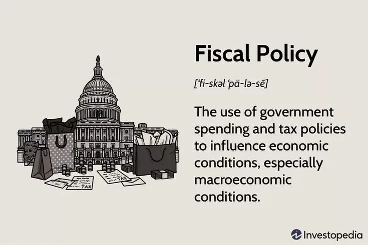
Fiscal policy refers to the decisions a government makes about how much to spend and how much to tax in order to influence the overall level of economic activity. It is one of the two primary tools governments use to manage their economies, the other being monetary policy.
When governments debate stimulus packages, austerity programs, tax cuts, or deficit spending, they are debating fiscal policy - decisions with real and often massive consequences for employment, growth, inequality, and the standard of living of millions of people.
The history of fiscal policy is a history of intellectual battles over the proper role of government in managing the business cycle, interspersed with natural experiments - recessions, wars, pandemics, and misguided policy interventions - that have progressively refined our understanding of when fiscal intervention works, when it fails, and why.
Fiscal Policy vs. Monetary Policy
The distinction between fiscal and monetary policy matters for understanding both how economies are managed and who holds the relevant power.
Monetary policy is conducted by central banks - in the United States, the Federal Reserve; in the eurozone, the European Central Bank - and works primarily through interest rates and the supply of money and credit.
A central bank cannot spend money on schools or cut income taxes; it operates through financial markets and the banking system.
Fiscal policy, by contrast, directly affects the real economy: government spending on infrastructure employs workers and builds roads; a cut in payroll taxes immediately puts more money in workers' paychecks.
But fiscal policy typically requires legislation, meaning it is subject to budget negotiations, parliamentary or congressional approval, and executive signature. This institutional sluggishness means fiscal policy often responds slowly to economic downturns.
"The boom, not the slump, is the right time for austerity at the Treasury." - John Maynard Keynes
Fiscal and monetary policy also interact in complicated ways. When fiscal policy involves large government borrowing, it can put upward pressure on interest rates, affecting monetary transmission.
In a low-interest-rate environment, as occurred after the 2008 financial crisis and during the COVID-19 pandemic, when the conventional tools of monetary policy became constrained by the zero lower bound, fiscal policy became the more important lever for managing aggregate demand.
The Zero Lower Bound Problem
When central banks have already cut short-term interest rates to near zero - as the Federal Reserve did after 2008 and again in 2020 - they lose their primary tool for stimulating the economy.
Quantitative easing (large-scale asset purchases) can supplement conventional monetary policy, but its effectiveness is more limited and contested. This creates situations where fiscal policy becomes the dominant macroeconomic stabilization tool by default.
The 2009 American Recovery and Reinvestment Act ($787 billion) and the 2020-2021 COVID relief packages (CARES Act at $2.2 trillion, American Rescue Plan at $1.9 trillion) were both enacted in environments where the Federal Reserve had already exhausted much of its conventional ammunition.
The scale and speed of fiscal response in 2020-2021 was unprecedented in peacetime - and the debate over whether it was well-sized continues to shape economic thinking.
Automatic Stabilizers: The Economy's Built-In Shock Absorbers
Automatic stabilizers are features of the tax and spending system that automatically change in ways that dampen economic fluctuations, without requiring any new political decisions. They are called automatic because they operate through built-in rules rather than discretionary action.
The primary examples are progressive income taxes and unemployment insurance. Consider what happens during a recession: as incomes fall and unemployment rises, the government automatically collects less in income tax (because people are earning less) and automatically pays out more in unemployment benefits (because more people qualify).
Both of these changes put money into the economy precisely when it is contracting. The government runs a larger deficit without anyone having to vote on it.
Conversely, during a boom, incomes rise, tax receipts increase, unemployment falls, and benefit payments decline. The government's deficit automatically shrinks or turns to surplus. This dampens the boom.
Automatic stabilizers are widely regarded as one of the most reliably effective tools of macroeconomic management precisely because they do not require the slow, contentious process of legislative action.
The degree of automatic stabilization in an economy depends on the size of the public sector, the progressivity of the tax system, and the generosity of social insurance programs.
European countries, which generally have larger welfare states and more progressive taxes, have stronger automatic stabilizers than the United States - a key reason why recessions tend to cause larger swings in US output.
| Economy | Automatic Stabilizer Strength | Primary Mechanism |
|---|---|---|
| Sweden, Denmark | Very high | Large public sector, generous unemployment benefits |
| Germany, France | High | Kurzarbeit (short-time work) schemes, social insurance |
| United Kingdom | Moderate-high | NHS, means-tested benefits |
| United States | Moderate | Unemployment insurance, progressive tax code |
| Japan | Moderate | Employment protection norms, smaller transfer programs |
The limitation of automatic stabilizers is that they are not sufficient for very deep recessions.
When a shock is large enough - as in the 2008-2009 financial crisis or the COVID-19 pandemic - governments may need to supplement with discretionary fiscal policy: deliberate new spending programs or tax cuts enacted specifically to combat the downturn.
The Keynesian Multiplier: How Much Does Government Spending Stimulate Growth?
The Keynesian fiscal multiplier is the ratio of the total change in economic output to the initial change in government spending (or taxes) that caused it. If the government spends an additional $1 billion on public works and the ultimate increase in GDP is $1.5 billion, the multiplier is 1.5.
The logic is that the initial spending creates income for workers and contractors, who spend some of that income on goods and services, generating income for further workers, who spend some of that, and so on through successive rounds of spending.
The size of the multiplier is one of the most contested empirical questions in macroeconomics. Classical economists argue that government spending crowds out private investment and consumption, potentially driving the multiplier toward zero or even below one.
Keynesian economists argue that during recessions, when private demand is weak and there is significant slack in the economy (unemployed workers, idle factories), the multiplier can be substantially above one because there is little crowding out to worry about.
The question moved from academic to urgently practical during the fiscal austerity programs of 2010-2012. Many European governments, under pressure from markets and institutions including the European Commission and IMF, sharply cut spending and raised taxes to reduce budget deficits.
The IMF had estimated fiscal multipliers at around 0.5 when approving these programs, implying that a $1 cut in spending would reduce GDP by only 50 cents.
In a widely cited 2013 paper, Olivier Blanchard and Daniel Leigh showed that the IMF had systematically underestimated multipliers, and that the actual multipliers during this period were between 1.5 and 1.7 in the eurozone. The programs were far more contractionary than anticipated.
Greece, which implemented the most severe austerity, saw its GDP fall by over 25 percent and its unemployment rate rise above 27 percent - consequences that substantially exceeded official projections at the time the programs were designed.
What Determines Multiplier Size?
The multiplier is not a fixed number. Research has identified several key factors that push it higher or lower:
Factors that increase the multiplier:
- Economic slack: High unemployment means spending does not crowd out other activity
- Liquidity constraints: Households unable to borrow spend additional income immediately
- Open economy vs. closed: More closed economies have higher multipliers (less leakage through imports)
- Type of spending: Infrastructure and direct government employment have higher multipliers than transfers
Factors that reduce the multiplier:
- Near-full employment: Government spending competes with private spending for scarce resources
- High indebtedness: Households anticipate future tax increases ("Ricardian equivalence")
- High trade openness: Stimulus leaks to trading partners
- Interest rate response: Central banks may raise rates to offset fiscal expansion
Crowding Out and Debt Sustainability
The crowding out hypothesis is a classical economics argument that government borrowing displaces private investment, potentially offsetting much or all of the stimulus effect of fiscal expansion.
The mechanism works through interest rates: when the government borrows heavily in credit markets, it competes with private borrowers for available savings, driving up interest rates. Higher interest rates make investment projects less profitable for businesses, so private investment falls.
The empirical evidence on crowding out is mixed and context-dependent. During deep recessions, when interest rates are already near zero and private investment is depressed because of weak demand, the crowding out effect is likely much smaller because additional government borrowing does not meaningfully increase competition for investable funds.
Debt sustainability is a related but distinct concern. Even if deficit spending is appropriate in the short run, a government that runs persistent deficits will accumulate debt. As debt grows, interest payments consume an increasing share of the budget, potentially requiring future tax increases or spending cuts.
In 2010, economists Carmen Reinhart and Kenneth Rogoff published a widely influential paper claiming to show that countries with debt-to-GDP ratios above 90 percent experienced significantly lower economic growth. This finding was cited extensively in favor of austerity programs.
However, in 2013, a graduate student named Thomas Herndon found coding errors and methodological problems in Reinhart and Rogoff's spreadsheet that had significantly distorted their results.
When corrected, the sharp threshold at 90 percent disappeared. This episode became emblematic of the risks of basing major policy decisions on a single empirical study.
| Debt-to-GDP Range | Reinhart-Rogoff Claim | Post-Correction Finding |
|---|---|---|
| Below 30% | Strong growth | Strong growth |
| 30-60% | Moderate growth | Moderate growth |
| 60-90% | Mild growth reduction | Mild growth reduction |
| Above 90% | Sharp growth reduction (~-0.1%) | Modest reduction (~-0.6% vs earlier claim) |
The Role of Interest Rates in Debt Sustainability
Whether government debt is sustainable depends critically on the relationship between the interest rate paid on debt (r) and the growth rate of the economy (g).
When r is less than g - as it was in most advanced economies for much of the 2010s - the economy grows faster than debt servicing costs, and relatively modest primary surpluses can stabilize debt-to-GDP ratios.
This insight, developed rigorously by Olivier Blanchard in his 2019 AEA presidential lecture, significantly changed how economists think about the costs of fiscal deficits.
The rise in global interest rates between 2022 and 2024 shifted this calculus. As central banks raised rates to combat inflation, the r-g relationship moved unfavorably for highly indebted governments.
Italy, Japan, and the United States all faced materially higher debt servicing costs, renewing debates about fiscal sustainability that had been dormant during the low-rate era.
Tax Policy: Progressivity and the Laffer Curve
Tax policy encompasses decisions about what to tax, how much to tax it, and how the burden is distributed across individuals and firms.
The two dominant philosophical positions on tax design are progressivity - taxing higher incomes or wealth at higher rates, on grounds of diminishing marginal utility and ability to pay - and neutrality or efficiency - minimizing the distortions that taxes create in economic behavior.
The Laffer Curve, popularized by economist Arthur Laffer and associated with supply-side economics, makes the observation that at a zero tax rate, the government collects no revenue, and at a 100 percent tax rate, no one has any incentive to earn taxable income, so revenue is also zero.
Somewhere between these extremes is a revenue-maximizing rate. The curve implies that if tax rates are above this optimum, cutting taxes could actually increase revenue by stimulating more economic activity.
The Laffer Curve argument is logically valid as a theoretical observation but empirically very uncertain. Estimating where actual tax rates sit relative to the revenue-maximizing point requires knowing the elasticity of taxable income - how much reported taxable income changes in response to a change in the tax rate.
Most empirical research suggests that for middle-income earners, this elasticity is quite low, meaning moderate tax increases do not significantly reduce economic activity.
Kansas provided a natural experiment in the early 2010s. Governor Sam Brownback implemented dramatic income tax cuts in 2012, explicitly invoking supply-side theory, predicting the cuts would trigger rapid economic growth that would restore revenues.
Instead, Kansas experienced persistent budget shortfalls, cuts to education and public services, and economic growth that lagged neighboring states. In 2017, the Republican-controlled Kansas legislature reversed the tax cuts over Brownback's veto.
The episode is regularly cited in debates about the limits of Laffer Curve reasoning in practice.
Tax Incidence: Who Really Bears the Burden?
Tax incidence refers to the question of who actually bears the economic burden of a tax, which is often different from who is legally required to pay it. This distinction between statutory incidence (legal liability) and economic incidence (actual burden) is one of the most important and underappreciated concepts in public finance.
The classic example is a payroll tax nominally split between employers and employees. The actual burden depends on the relative elasticities of supply and demand in the labor market - that is, on how responsive workers and employers are to wage changes.
If labor supply is relatively inelastic (workers must work regardless of wages), workers end up bearing most of the burden even of the employer's share, because employers respond to higher labor costs by paying lower gross wages.
Similarly, corporate income taxes are nominally paid by corporations, but who actually bears the burden depends on how capital and labor markets adjust.
If capital can move internationally in response to higher taxation, companies may shift production to lower-tax jurisdictions, reducing the capital stock and wages in the higher-tax country.
In this scenario, workers end up bearing a substantial fraction of the corporate tax burden through lower wages.
| Tax Type | Statutory Payer | Likely Actual Burden |
|---|---|---|
| Payroll tax (employer share) | Employer | Partly workers (through lower wages) |
| Corporate income tax | Corporation | Partly workers, partly shareholders |
| Sales tax | Consumer at point of sale | Consumer and partly producer |
| Property tax (land) | Landowner | Primarily landowner (fixed supply) |
| Property tax (improvements) | Landowner | Partly shifted to tenants/consumers |
The Global Minimum Corporate Tax
The global minimum corporate tax is an agreement, reached in principle in October 2021 under the auspices of the OECD and G20, to impose a minimum effective corporate income tax rate of 15 percent on the profits of large multinational corporations.
By early 2024, over 140 countries had agreed to the framework, and many had begun implementing it in domestic legislation.
The background is the phenomenon of tax competition and base erosion. Over the past thirty years, countries have competed aggressively for corporate investment by offering low tax rates, preferential regimes, and favorable tax rulings.
Ireland offered a 12.5 percent corporate tax rate, attracting the European headquarters of many US technology companies.
Various small jurisdictions offered structures that allowed multinational companies to shift profits to low-tax or zero-tax locations while conducting their real economic activities elsewhere.
The OECD estimated that governments collectively lose between $100 billion and $240 billion annually in corporate tax revenue through these mechanisms.
The 15 percent minimum works through a top-up mechanism: if a multinational pays less than 15 percent effective tax in a given jurisdiction, the home country of the parent company can collect additional tax to bring the total to 15 percent.
This removes the incentive to shift profits to zero-tax jurisdictions because the tax advantage disappears.
Critics argue the 15 percent rate is too low and that the many exceptions and carve-outs in the agreement limit its effectiveness. Advocates say it is a significant step toward ending the race to the bottom in corporate taxation, even if an imperfect one.
Fiscal Policy and Inequality
Beyond aggregate stabilization, fiscal policy is a primary tool for affecting the distribution of income and wealth. The combination of progressive taxation and targeted social transfers is one of the most significant determinants of post-tax income inequality across countries.
Research by economists at the OECD and IMF has documented that fiscal systems in most advanced economies redistribute substantially. In the United States in 2023, the Gini coefficient for market income (before taxes and transfers) was approximately 0.50 - extremely high by international standards.
After taxes and transfers, the post-fiscal Gini fell to roughly 0.39. This reduction of 0.11 Gini points represents an enormous absolute redistribution, though the U.S. fiscal system redistributes less than most peer economies.
"Fiscal policy operates as the primary mechanism by which democratic societies manage the tension between market-generated inequality and social cohesion. Every budget is, at its core, a statement of distributive values expressed in numbers." - IMF Fiscal Monitor, 2017
The Nordic model - high progressive taxation funding universal public services (healthcare, education, childcare, eldercare) - produces among the lowest inequality ratios in the world while maintaining competitive economies.
This outcome suggests that the trade-off between efficiency and equality in tax design is less stark than classical economics sometimes implies, provided the spending is directed toward investments in human capital and economic security that also enhance productivity.
COVID-19 and the Largest Peacetime Fiscal Expansion
The COVID-19 pandemic produced the largest peacetime fiscal expansion in modern history. According to the IMF, global fiscal support in 2020 reached approximately $16 trillion, or around 15 percent of global GDP, combining direct spending measures, tax deferrals, equity injections, and loan guarantees.
The United States, where COVID fiscal response was particularly large, ran a deficit of 15.8 percent of GDP in 2020 - the largest since World War II.
The combination of direct payments ($1,200 per adult in 2020, $1,400 in 2021), expanded unemployment benefits ($600 per week supplement in 2020), and business support through the Paycheck Protection Program was unprecedented in speed and scale.
The subsequent inflation surge - U.S. CPI peaked at 9.1 percent year-over-year in June 2022 - became the central debate about whether the fiscal response, particularly the 2021 American Rescue Plan, was appropriately sized or excessive given the economy's state at that point.
Economists Lawrence Summers and Olivier Blanchard warned in early 2021 that the ARP was likely to overheat the economy; Treasury Secretary Janet Yellen and CEA chair Cecilia Rouse argued the risks of undershooting were greater.
The inflation that followed prompted significant reconsideration of stimulus sizing in academic and policy circles.
Practical Implications: What Fiscal Policy Can and Cannot Do
Understanding fiscal policy matters for anyone who votes, invests, runs a business, or simply wants to understand why economic conditions change over time. Several practical lessons emerge from the research.
Fiscal policy works best during deep recessions. When the economy is substantially below capacity - high unemployment, idle capital, depressed private investment - fiscal stimulus is most effective because crowding out is minimized. The same stimulus during a boom can be counterproductive, generating inflation rather than growth.
The composition of spending and tax changes matters as much as their size. Public investment (infrastructure, research, education) tends to have higher multipliers than transfer payments, which have higher multipliers than upper-income tax cuts.
The distributional and dynamic effects of fiscal choices are inseparable from their aggregate demand effects.
Institutional constraints shape what is politically achievable. Automatic stabilizers operate precisely because they circumvent the legislative process. Discretionary fiscal policy often arrives too late, is too small, or is designed for political rather than economic goals.
The history of economic stimulus packages reveals a persistent tendency to undersize interventions out of concern about deficits, while the empirical evidence suggests undersized stimulus prolongs recessions.
The debt sustainability question cannot be ignored. While debt limits have proven more flexible than earlier research suggested, and while interest rates near zero changed the calculus substantially, the long-run trajectory of government finances matters for investment confidence and intergenerational equity.
The appropriate question is not whether fiscal deficits are ever permissible but whether borrowing is being used for purposes (public investment, crisis response) that generate returns commensurate with debt costs.
Fiscal policy sits at the intersection of economics, politics, and social choice.
Its technical dimensions - multiplier estimates, debt sustainability thresholds, tax incidence calculations - matter enormously, but they do not resolve the underlying questions about distribution, risk-sharing, and the proper scope of collective action that drive most fiscal debates.
Those questions are ultimately political, and understanding the economics is a prerequisite for engaging them honestly.
Frequently Asked Questions
What is fiscal policy and how does it differ from monetary policy?
Fiscal policy refers to the decisions a government makes about how much to spend and how much to tax in order to influence the overall level of economic activity. When the government spends more than it collects in taxes, it runs a fiscal deficit. When it collects more than it spends, it runs a surplus. The size and composition of that gap - and how it is financed - has significant effects on employment, inflation, economic growth, and income distribution.The distinction from monetary policy is important. Monetary policy is conducted by central banks (in the United States, the Federal Reserve; in the eurozone, the European Central Bank) and works primarily through interest rates and the supply of money and credit. A central bank cannot spend money on schools or cut income taxes; it operates through financial markets and the banking system. Fiscal policy, by contrast, directly affects the real economy: government spending on infrastructure builds roads and employs workers; a cut in payroll taxes immediately puts more money in workers’ paychecks.The two are complementary but often operate with different institutional timelines and political constraints. Central banks can adjust interest rates at regular scheduled meetings, sometimes with rapid effect on financial conditions. Fiscal policy typically requires legislation, meaning it is subject to the full political process of budget negotiations, parliamentary or congressional approval, and executive signature. This institutional sluggishness means fiscal policy often responds slowly to economic downturns.Fiscal and monetary policy also interact in sometimes complicated ways. When fiscal policy involves large government borrowing, it can put upward pressure on interest rates, affecting the ease of monetary transmission. In a low-interest-rate environment, as occurred after the 2008 financial crisis and during the COVID-19 pandemic, the conventional tools of monetary policy can become constrained, making fiscal policy the more important lever for managing aggregate demand. The coordination - or lack thereof - between fiscal and monetary authorities is a recurring theme in macroeconomic policy debates.
What are automatic stabilizers and how do they smooth economic cycles?
Automatic stabilizers are features of the tax and spending system that automatically change in ways that dampen economic fluctuations, without requiring any new political decisions. They are called automatic because they operate through built-in rules rather than discretionary action.The primary examples are progressive income taxes and unemployment insurance. Consider what happens during a recession: as incomes fall and unemployment rises, the government automatically collects less in income tax (because people are earning less) and automatically pays out more in unemployment benefits (because more people qualify). Both of these changes put money into the economy precisely when it is contracting. The government runs a larger deficit without anyone having to vote on it. Conversely, during a boom, incomes rise, tax receipts increase, unemployment falls, and benefit payments decline. The government’s deficit automatically shrinks or turns to surplus. This dampens the boom.Automatic stabilizers are widely regarded as one of the most reliably effective tools of macroeconomic management, precisely because they do not require the slow, contentious process of legislative action. They are also symmetric: they work in recessions and booms alike. The degree of automatic stabilization in an economy depends on the size of the public sector, the progressivity of the tax system, and the generosity of social insurance programs. European countries, which generally have larger welfare states and more progressive taxes, have stronger automatic stabilizers than the United States. This is one reason why recessions tend to cause larger swings in US output relative to European economies with similar shocks.The limitation of automatic stabilizers is that they are not sufficient for very deep recessions. When a shock is large enough - as in the 2008-2009 financial crisis or the COVID-19 pandemic - the automatic response may be inadequate and governments may need to supplement it with discretionary fiscal policy: deliberate new spending programs or tax cuts enacted specifically to combat the downturn. The interaction between automatic and discretionary fiscal policy, and the appropriate size and timing of discretionary interventions, is one of the central questions of applied macroeconomics.
What is the Keynesian multiplier and how large is it?
The Keynesian fiscal multiplier is the ratio of the total change in economic output to the initial change in government spending (or taxes) that caused it. If the government spends an additional \(1 billion on public works and the ultimate increase in GDP is \)1.5 billion, the multiplier is 1.5. The logic is that the initial spending creates income for workers and contractors, who spend some of that income on goods and services, generating income for further workers, who spend some of that, and so on through successive rounds of spending. The multiplier captures the sum of this cascading effect.The size of the multiplier is one of the most contested empirical questions in macroeconomics. Classical economists argue that government spending crowds out private investment and consumption, potentially driving the multiplier toward zero or even below one. Keynesian economists argue that during recessions, when private demand is weak and there is significant slack in the economy (unemployed workers, idle factories), the multiplier can be substantially above one because there is little crowding out to worry about.The question moved from academic to urgently practical during the fiscal austerity programs of 2010-2012. Many European governments, under pressure from markets and institutions including the European Commission and IMF, sharply cut spending and raised taxes to reduce budget deficits. The IMF had estimated fiscal multipliers at around 0.5 when approving these programs, implying that a $1 cut in spending would reduce GDP by only 50 cents. In a widely cited 2013 paper, Olivier Blanchard and Daniel Leigh showed that the IMF had systematically underestimated multipliers, and that the actual multipliers during this period were between 1.5 and 1.7 in the eurozone. The programs were far more contractionary than anticipated. Greece, which implemented the most severe austerity, saw its GDP fall by over 25 percent and its unemployment rate rise above 27 percent. The multiplier debate had enormous real-world consequences.
What is the debate over crowding out and debt sustainability?
The crowding out hypothesis is a classical economics argument that government borrowing displaces private investment, potentially offsetting much or all of the stimulus effect of fiscal expansion. The mechanism works through interest rates: when the government borrows heavily in credit markets, it competes with private borrowers for available savings, driving up interest rates. Higher interest rates make investment projects less profitable for businesses, so private investment falls. In the most extreme version of this argument, complete crowding out occurs: every dollar of government spending displaces exactly one dollar of private spending, leaving total output unchanged.The empirical evidence on crowding out is mixed and context-dependent. In normal times, with relatively full employment and financial markets functioning well, some crowding out probably does occur, though estimates of its magnitude vary widely. During deep recessions, when interest rates are already near zero and private investment is depressed because of weak demand, the crowding out effect is likely much smaller because additional government borrowing does not meaningfully increase competition for investable funds. This is why most economists supported fiscal stimulus during the 2008-2009 recession and the 2020 COVID shock.Debt sustainability is a related but distinct concern. Even if deficit spending is appropriate in the short run, a government that runs persistent deficits will accumulate debt. As debt grows, interest payments consume an increasing share of the budget, potentially requiring future tax increases or spending cuts. In 2010, economists Carmen Reinhart and Kenneth Rogoff published a widely influential paper claiming to show that countries with debt-to-GDP ratios above 90 percent experienced significantly lower economic growth. This finding was cited extensively in favor of austerity programs. However, in 2013, a graduate student named Thomas Herndon found coding errors and methodological problems in Reinhart and Rogoff’s spreadsheet that had significantly distorted their results. When corrected, the sharp threshold at 90 percent disappeared. This episode became emblematic of the risks of basing major policy decisions on a single empirical study, and it reinvigorated debate about how much weight to give debt-to-GDP ratios in fiscal policy decisions.
How does tax policy work and what are the key debates around progressivity and the Laffer Curve?
Tax policy encompasses decisions about what to tax, how much to tax it, and how the burden is distributed across individuals and firms. The two dominant philosophical positions on tax design are progressivity - taxing higher incomes or wealth at higher rates, on grounds of diminishing marginal utility and ability to pay - and neutrality or efficiency - minimizing the distortions that taxes create in economic behavior.The Laffer Curve, popularized by economist Arthur Laffer and associated with supply-side economics, makes the observation that at a zero tax rate, the government collects no revenue, and at a 100 percent tax rate, no one has any incentive to earn taxable income, so revenue is also zero. Somewhere between these extremes is a revenue-maximizing rate. The curve implies that if tax rates are above this optimum, cutting taxes could actually increase revenue by stimulating more economic activity. This argument was used to justify the Reagan tax cuts of 1981 and similar policies in subsequent decades.The Laffer Curve argument is logically valid as a theoretical observation but empirically very uncertain. Estimating where actual tax rates sit relative to the revenue-maximizing point requires knowing the elasticity of taxable income - how much reported taxable income changes in response to a change in the tax rate. Most empirical research suggests that for middle-income earners, this elasticity is quite low, meaning moderate tax increases do not significantly reduce economic activity. High-income earners show somewhat higher elasticities, partly because they have more legal avenues for tax planning, but even here the evidence does not support the strong claim that rate reductions will pay for themselves through revenue growth.Kansas provided a natural experiment in the early 2010s. Governor Sam Brownback implemented dramatic income tax cuts in 2012, explicitly invoking supply-side theory, predicting the cuts would trigger rapid economic growth that would restore revenues. Instead, Kansas experienced persistent budget shortfalls, cuts to education and public services, and economic growth that lagged neighboring states. In 2017, the Republican-controlled Kansas legislature reversed the tax cuts over Brownback’s veto. The episode is regularly cited in debates about the limits of Laffer Curve reasoning in practice.
What is tax incidence and why does it matter for policy?
Tax incidence refers to the question of who actually bears the economic burden of a tax, which is often different from who is legally required to pay it. This distinction between statutory incidence (legal liability) and economic incidence (actual burden) is one of the most important and underappreciated concepts in public finance.The classic example is a payroll tax nominally split between employers and employees. Both sides pay a share of the total. But economic analysis shows that the actual burden depends on the relative elasticities of supply and demand in the labor market - that is, on how responsive workers and employers are to wage changes. If labor supply is relatively inelastic (workers must work regardless of wages), workers end up bearing most of the burden even of the employer’s share, because employers respond to higher labor costs by paying lower gross wages. If labor demand is inelastic (firms must hire regardless of wage), employers bear more of the burden. The statutory split between employer and employee contributions is economically largely irrelevant.Similarly, corporate income taxes are nominally paid by corporations, but who actually bears the burden depends on how capital and labor markets adjust. If capital can move internationally in response to higher taxation, companies may shift production to lower-tax jurisdictions, reducing the capital stock and wages in the higher-tax country. In this scenario, workers end up bearing a substantial fraction of the corporate tax burden through lower wages - a result that challenges progressive intuitions about corporate taxation.Sales taxes are nominally paid by consumers but some portion may be borne by producers if demand is elastic and consumers reduce purchases substantially when prices rise. Property taxes are largely borne by landowners for the land component (land supply is fixed) but may be partly shifted to renters or consumers for the improvements component. Getting tax incidence right matters enormously for designing fair and effective tax policy, and it is why economists often reach different conclusions about the distributional effects of taxes than simple statutory analysis would suggest.
What is the global minimum corporate tax and why was it adopted?
The global minimum corporate tax is an agreement, reached in principle in October 2021 under the auspices of the OECD and G20, to impose a minimum effective corporate income tax rate of 15 percent on the profits of large multinational corporations. By early 2024, over 140 countries had agreed to the framework, and many had begun implementing it in domestic legislation. It represents the most significant restructuring of international corporate taxation in decades.The background is the phenomenon of tax competition and base erosion. Over the past thirty years, countries have competed aggressively for corporate investment by offering low tax rates, preferential regimes, and favorable tax rulings. Ireland offered a 12.5 percent corporate tax rate, attracting the European headquarters of many US technology companies. Various small jurisdictions - the Cayman Islands, Bermuda, Luxembourg, the Netherlands - offered structures that allowed multinational companies to shift profits to low-tax or zero-tax locations while conducting their real economic activities elsewhere. Economists call this profit shifting and base erosion. The OECD estimated that governments collectively lose between \(100 billion and \)240 billion annually in corporate tax revenue through these mechanisms.The political consensus for action built through the 2010s as major technology companies - Google, Apple, Facebook, Amazon - became notorious for paying very low effective tax rates despite enormous profits in high-tax countries. Public anger combined with revenue pressure on governments managing COVID-19 recovery packages created the political conditions for agreement.The 15 percent minimum works through a top-up mechanism: if a multinational pays less than 15 percent effective tax in a given jurisdiction, the home country of the parent company (and in some cases other countries where it operates) can collect additional tax to bring the total to 15 percent. This removes the incentive to shift profits to zero-tax jurisdictions because the tax advantage disappears. Critics argue the 15 percent rate is too low and that the many exceptions and carve-outs in the agreement limit its effectiveness. Advocates say it is a significant step toward ending the race to the bottom in corporate taxation, even if an imperfect one.